Accelerating encrypted analytics on confidential data by 20x
Summary: In this engineering blog post, we discuss technical details surrounding Opaque Systems’ closed source version of Opaque SQL. This project extends Apache Spark SQL with a physical operator layer that runs inside hardware enclaves to protect confidential data in use. However, this latest iteration contains physical operators that are vectorized and are being performed over data stored in columnar batches. The result is a SQL engine over 20x faster than the previous version and within 2x the performance of vanilla, unencrypted Spark SQL. Protecting confidential data in use has never been more efficient and practical for large-scale workloads.
Introduction
Opaque SQL is an encrypted analytics engine built on top of Apache Spark SQL that replaces the plaintext query execution layer with execution inside hardware enclaves. This successfully protects the confidentiality of the data in use, but how does this new layer actually work? In this blog post, we’ll first take a look at our original approach (interpreted, row-based query execution) and its shortcomings. Then, we’ll dive into how our new technique, vectorization, overcomes these limitations to enable significant performance improvements.
Interpreted query execution
At the implementation level, Opaque SQL uses an interpreted, row-by-row execution engine to evaluate a query. Each operation executes on a single row at a time, which is quite inefficient due to the overhead of dynamic dispatch:
Combined with the overhead of using enclaves, this implementation considerably impacts the performance of Opaque SQL. Our benchmarking numbers, even working with data as small as 1GB, lag behind vanilla Spark SQL. This had to be addressed, as a key feature of Opaque Systems’ product is to be able to run at scale on terabytes of data.
Improving execution
Instead of row-based, interpreted execution, modern database management systems (DBMSs) rely on two techniques for fast query execution: code generation and vectorization.
For a given query, the DBMS generates code that should be used to execute it at runtime. As a result, there is no overhead of dynamic dispatch since the generated code is specialized for each query.
Vectorization
Vectorization involves using batched execution that allows computation to be performed on multiple fields in the same column using only a single operation. There is still dynamic dispatch, but the interpretation overhead is amortized since it happens only once per input.
In practice, these two techniques exhibit different tradeoffs, but the overall benchmark performance is similar (see this paper for numbers). However, when deciding which one to use for our purpose, a clear winner emerges.
Because of the current restrictions regarding running dynamic executables in hardware enclaves, we cannot dynamically generate code inside an enclave and link it to execute during runtime. There would have to be multiple build steps, and the client would also need a way to get the query-specific executable (in a trusted manner) for attestation. Because of this complication, we chose vectorized, interpreted execution as our performance improving workhorse.
There are many existing, high-quality vectorized SQL engines. For the best utilization of developer time and to take advantage of existing open source, we decided to port over the execution layer of DuckDB, a high-performance OLAP database written in C++. DuckDB is lightweight and is designed to be an embeddable database.
Technical challenges
Porting and adapting DuckDB for Opaque SQL involved a number of technical challenges: we illustrate two such obstacles below.
Overcoming differences between planning and execution layers
Using DuckDB’s execution layer imposed some restrictions on the variety of physical plans we can actually execute. In this section, we highlight a difference in planning the TPC-H 7 query. Because it is possible to modify Spark’s planning without forking the repository, we settled on modifying the planning layer instead of the execution layer to overcome these differences.
Consider the following equi-join that has an additional condition (n1.n_name = 'FRANCE' and n2.n_name = 'GERMANY') or (n1.n_name = 'GERMANY' and n2.n_name = 'FRANCE'). Spark’s planning includes this entire condition in the join step:
However, DuckDB’s physical hash join operator only works with comparison conditions between columns, e.g., key1 > key2, key1 = key2 etc…
To overcome the incompatibility in this particular example, we modified our planning to perform a filter on this join condition after the actual hash join. The modified step looks like this:
This is a key difference from our non-vectorized code, where our planning layer for the most part just uses the default for vanilla Spark SQL.
It’s possible to achieve the same result with different plans. For example, because the condition only contains columns from the right table in the join, we can schedule the filter on that table before the join. This will be more efficient than the illustrated plan; filter pushdown is a common optimization included in the planning stage to reduce the amount of data processed in later steps. Considering these optimizations was not done in this first version of the vectorized engine, but is something we will think about when improving performance in future iterations.
Extending DuckDB’s execution to work in a distributed setting
DuckDB is designed for single machine processing of data, whereas Spark SQL is a distributed computing engine that executes on multiple partitions of data spread out across different executors. Therefore, porting DuckDB to the distributed setting is not as straightforward as a one-to-one mapping. We needed to define our own physical operators that require a shuffle (e.g., join, aggregation, order by).
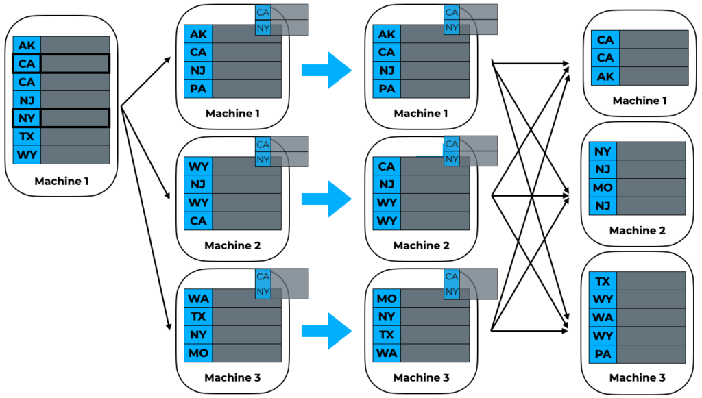
Consider a basic hash join on left.state == right.state:
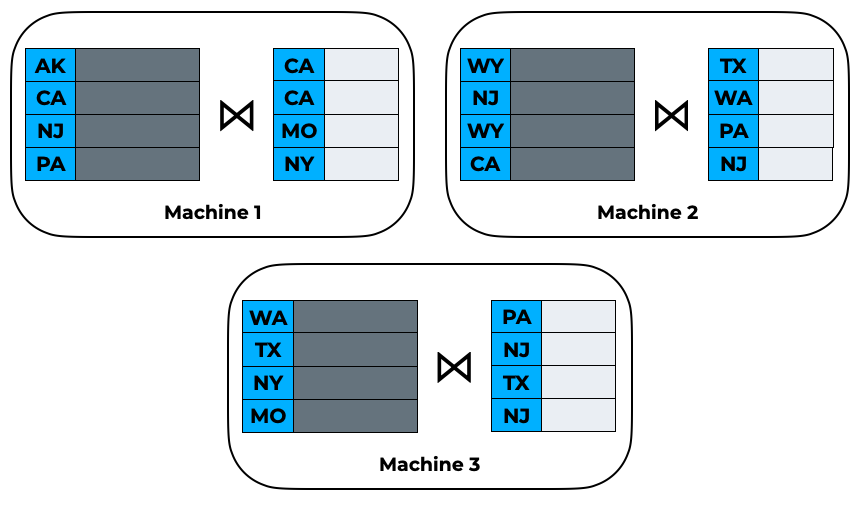
If we naively use DuckDB to perform a join on each individual partition, the result will be incorrect! The left data may contain keys that are found in the right data on a different partition — these will not be matched. It becomes necessary to perform a hash partitioning before the actual join step so that the relevant records are co-located on the same machine:
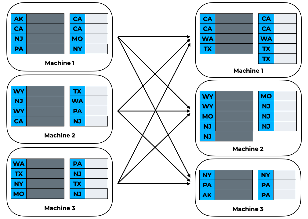
After the hash partition step, we see that all keys are now distributed in the same partition across left and right sides of the join. Therefore, we can now perform the join on each individual partition.
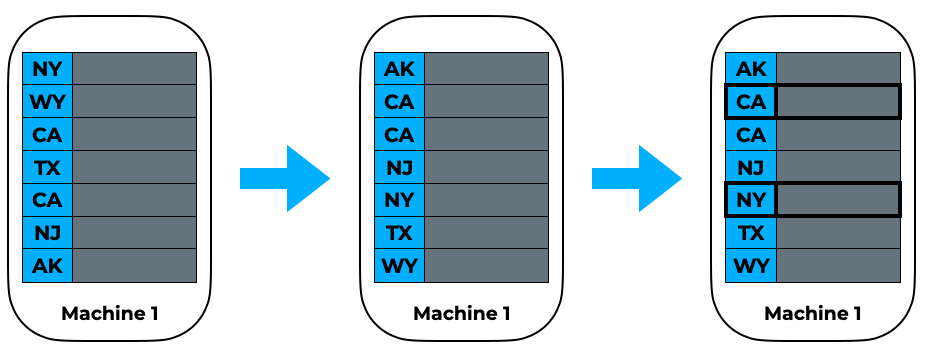
As another, slightly more complicated, example, consider the input to a basic distributed sort on the state column:
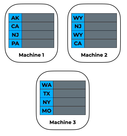
If we perform a local sort on each partition, the result will again be incorrect, since the input partitions may contain keys that should be in different partitions in the final result. For this, we go through a 3-step process to perform a range partitioning:
Step 1
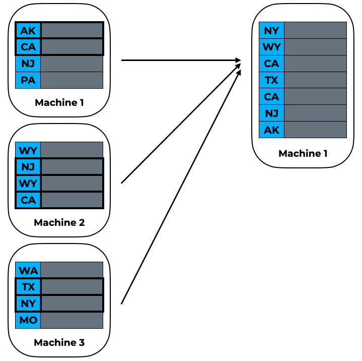
We collect a random sample of sort keys, and parcel that out to a single worker. Because this is just a sample, we can assume that aggregating the values over all data partitions into one partition will not be too costly.
Step 2
Using the sample, find some range bounds that would be a strong estimate of evenly distributing where a random element in the global data would go. This is done by first sorting locally, then evenly placing bounds depending on the total number of partitions.
Step 3
Broadcast the range bounds to each original data partition, perform a local sort on each partition, then place a given element in each partition into the output partition corresponding to which range bound it falls into. Once this final step is complete, it is easy to see that a local sort in each partition will now create the correct result!
DuckDB had no need for such operations, so it was up to us to efficiently design these prequel steps and insert them where needed.
Performance evaluation
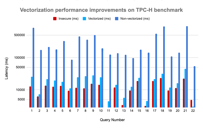
To evaluate our new system, we ran the entire TPC-H benchmark, comparing vanilla Spark SQL vs. non-vectorized Opaque SQL vs. vectorized Opaque SQL.
Cluster specifications
We used 3 Azure DC4ds_v3 VMs, each with the following specifications:
- 4 cores
- 16 GiB memory
- Up to 16 GiB enclave page cache (EPC) size
Spark configurations
- spark.driver.memory: 3g
- spark.driver.cores: 1
- spark.executor.memory: 2g
- spark.executor.instances: 12
- spark.executor.cores: 1
- spark.default.parallelism: 12
- spark.sql.shuffle.partitions: 12
Benchmark results (3 GB files)
Future work
We are very excited about the work done so far in building a scalable, fast, encrypted SQL analytics engine; that’s not to say there isn’t room for further improvements.
Currently, vectorized Opaque SQL has limited functionality: window functions and rollup/cube are some examples of operators not yet supported. For our goal of full TPC-DS support in the near future, we are currently working on implementing these operators.
When porting over DuckDB initially, we discovered some incompatibilities between the threading library used in DuckDB and that supported by the enclave SDK we are using. We can enhance the performance of our execution layer, and enable another layer of parallelism, by resolving these incompatibilities.
Our planning layer is still very similar to that of Catalyst, Spark SQL’s default planner. We can further optimize this layer by building around DuckDB’s physical operators — using these concrete building blocks, how can we construct a query plan to best take advantage of their implementations and associated complexities?
If any of these topics interest you, we’d love to chat! Please see our career page for open positions. You can also visit our open source and join our Slack channel for any questions you may have.